SGD Variants
Posted on Thu 29 March 2018 in Basics
To train our neural net we detailed the algorithm of Stochastic Gradient Descent in this article and implemented it in this one. To make it easier for our model to learn, there are a few ways we can improve it.
Vanilla SGD
Just to remember what we are talking about, the basic algorithm consists in changing each of our parameter this way
where \(p_{t}\) represents one of our parameters at a given step \(t\) in our loop, \(g_{t}\) the gradient of the loss with respect to \(p_{t}\) and \(\hbox{lr}\) is an hyperparameter called learning rate. In a pytorch-like syntax, this can be coded:
for p in parameters:
    p = p - lr * p.grad
Momentum
This amelioration is based on the observation that with SGD, we don't really manage to follow the line down a steep ravine, but rather bounce from one side to the other.
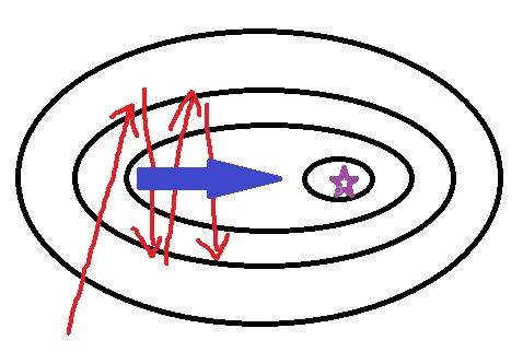
In this case, we would go faster by following the blue line. To do this, we will take some kind of average over the gradients, by updating our parameters like this:
where \(\beta\) is a new hyperparameter (often equals to 0.9). More details here. In code, this would look like:
for p in parameters:
    v[p] = beta * v[p] + lr * p.grad
    p = p - v[p]
where we would store the values of the various variables v in a dictionary indexed by the parameters.
Nesterov
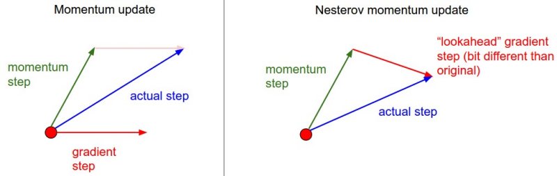
Nesterov is an amelioration of momentum based on the observation that in the momentum variant, when the gradient start to really change direction (because we have passed our minimum for instance), it takes a really long time for the averaged values to realize it. In this variant, we first take the jump from \(p_{t}\) to \(p_{t} - \beta v_{t-1}\) then we compute the gradient. To be more precise, instead of using \(g_{t} = \overrightarrow{\hbox{grad}} \hbox{ loss}(p_{t})\) we use
This picture (coming from this website) explains the difference with momentum
In code, this needs to have a function that reevaluates the gradients after we do this first step.
for p in parameters:
    p1 = p - beta v[p]
model.reevaluate_grads()
for p in parameters
    v[p] = beta * v[p] + lr * p.grad
    p = p - v[p]
RMS Prop
This is another variant of SGD that has been proposed by Geoffrey Hinton in this course It suggests to divide each gradient by a moving average of its norm. More specifically, the update in this method looks like this:
where \(\beta\) is a new hyperparameter (usually 0.9) and \(\epsilon\) a small value to avoid dividing by zero (usually \(10^{-8}\)). It's easily coded:
for p in parameters:
    n[p] = beta * n[p] + (1-beta) * p.grad ** 2
    p = p - lr * p.grad / np.sqrt(n[p] + epsilon)
Adam
Adam is a mix between RMS Prop and momentum. Here is the full article explaining it. The update in this method is:
where \(\beta_{1}\) and \(\beta_{2}\) are two hyperparameters, the advised values being 0.9 and 0.999. We go from \(m_{t}\) to \(\widehat{m_{t}}\) to have smoother first values (as we explained it when we implemented the learning rate finder). It's same for \(n_{t}\) and \(\widehat{n_{t}}\).
We can code this quite easily:
for p in parameters:
    m[p] = beta1 * m[p] + (1-beta1) * p.grad
    n[p] = beta2 * n[p] + (1-beta2) * p.grad ** 2
    m_hat = m[p] / (1-beta1**t)
    n_hat = n[p] / (1-beta2**t)
    p = p - lr * m_hat / np.sqrt(n_hat + epsilon)
Both RMS Prop and Adam have the advantage of smoothing the gradients with this moving average of the norm. This way, we can pick a higher learning rate while avoiding the phenomenon where gradients were exploding.
In conclusion
To get a sense on how these methods are all doing compared to the other, I've applied each of them on the digit classifier we built in pytorch and plotted the smoothed loss ( as described when we implemented the learning rate finder) for each of them.
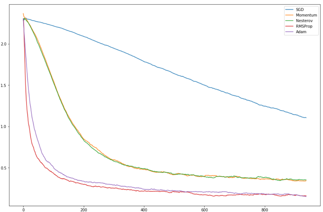
This is the loss as we go through our mini-batches with the same initial model. All variants are better than vanilla SGD, but it's probably because it needed more time to get to a better stop. What's interesting is that RMSProp and Adam tend to get the loss really low extremely fast.