What Is Deep Learning?

Posted on Tue 13 March 2018 in Basics

What is deep learning? It's a class of algorithms where you train something called a neural net to complete a specific task. Let's begin with a general overview and we will dig into the details in subsequent articles.

A neural net

To some extent, a neural net is an attempt by engineers to get a computer to replicate the behavior of our brain. A neuron in our brain gets a .

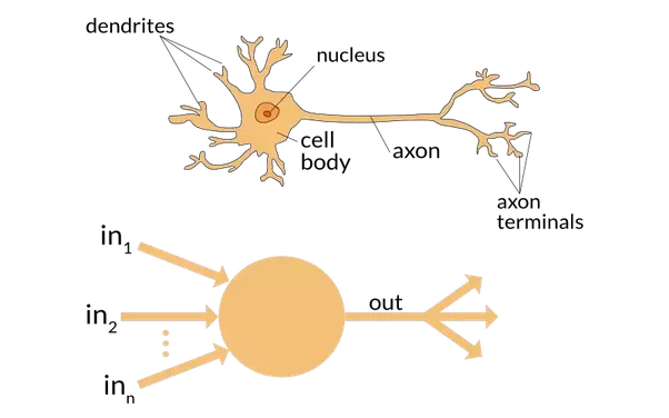
A model of that is to consider a structure getting a certain number of entries, each of them having a weight attributed to them. If this neuron as \(n\) entries that are \(x_{1},\dots,x_{n}\), with the weights \(w_{1},\dots,w_{n}\), we consider the sum of the inputs multiplied by the weight to compute the output:

\begin{equation*} y = f \left ( w_{1}x_{1} + \cdots + w_{n}x_{n} \right ) \end{equation*}

or in a more compact way

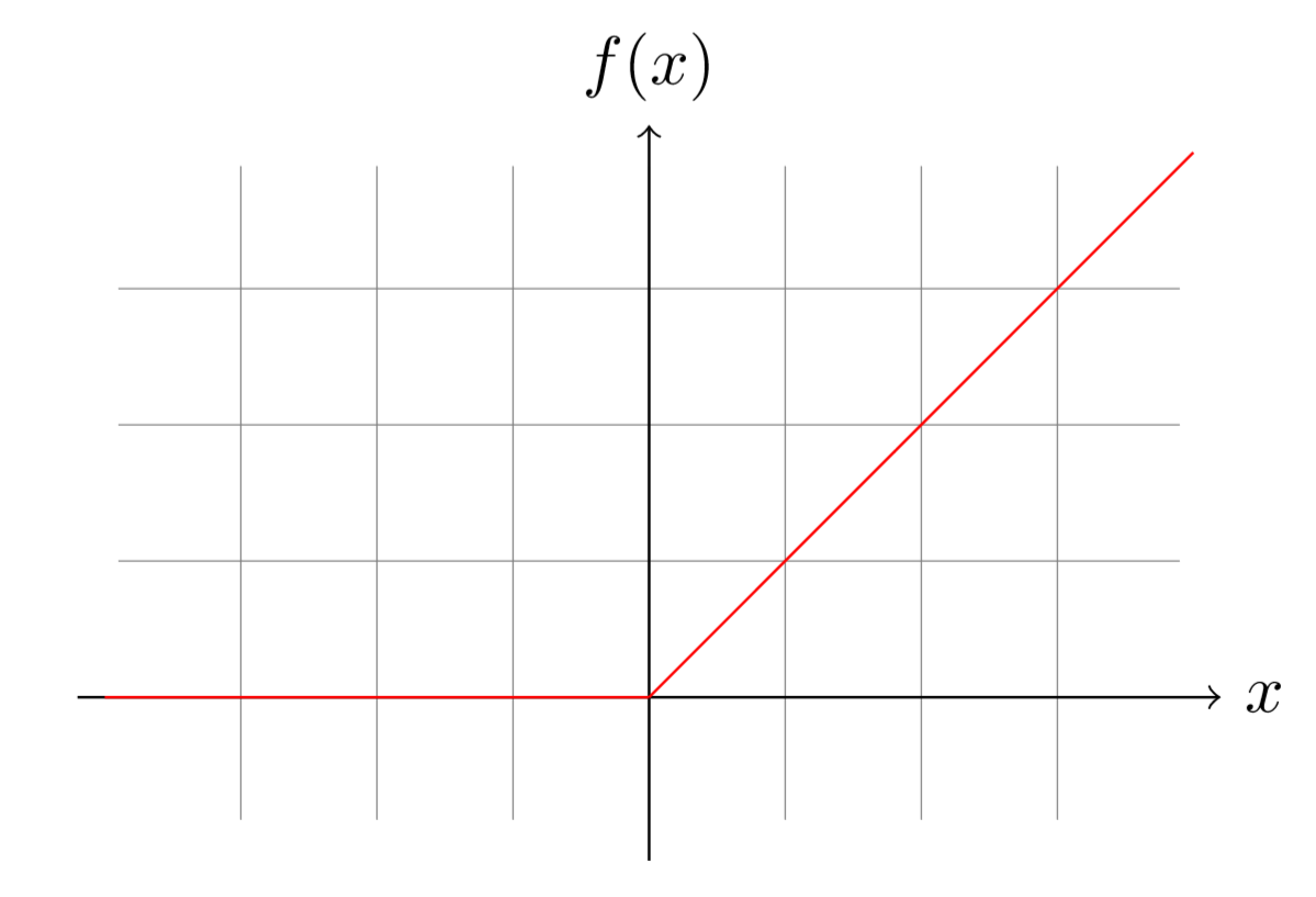
\begin{equation*} y = f \left ( \sum_{i=1}^{n} w_{i} x_{i} \right ). \end{equation*}

Here \(y\) is the output and \(f\) a function called the activation function. A few classical activation functions are the rectified linear unit (ReLU), the sigmoid function or the hyperbolic tangent function:

\begin{equation*} \hbox{ReLU}(x) = \max(0,x) \end{equation*}

\begin{equation*} \sigma(x) = \frac{\mathrm{e}^{x}}{1+\mathrm{e}^{x}} \end{equation*}

\begin{equation*} \hbox{tanh}(x) = \frac{\mathrm{e}^{x} - \mathrm{e}^{-x}}{\mathrm{e}^{x} + \mathrm{e}^{-x}} \end{equation*}

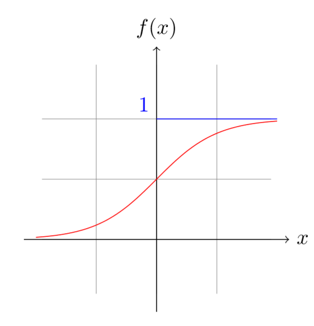
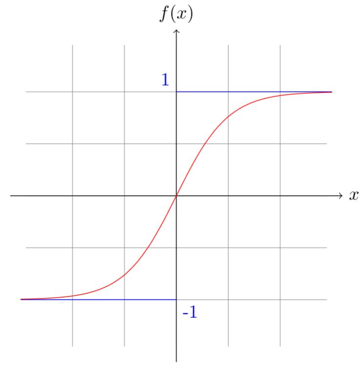
The function \(\hbox{tanh}\) is actually a sigmoid that we enlarged and translated to go from -1 to 1. To do this, we just have to multiply the sigmoid by 2 (the range between -1 and 1) then subtract 1:

\begin{equation*} \hbox{tanh}(x) = 2 \sigma(2x) - 1 \end{equation*}

These three functions are just the three most popular, but we could take any function, as long as it's non-linear and easy to differentiate (for reasons we will see later).

One last parameter we usually consider in our neuron is something called a bias, that is added to the weighted sum of the inputs before going into the activation function.

\begin{equation*} y = f \left ( \sum_{i=1}^{n} w_{i} x_{i} + b \right ). \end{equation*}

If we consider the case of a ReLU activation function (which basically replaces the negative by zero), the opposite of this bias is then the minimum value to reach to get an output that isn't nil.

So that's one neuron. In a neural net, we have quite a few of them, regrouped in what we call layers. An example of neural net with a single layer would look like this:

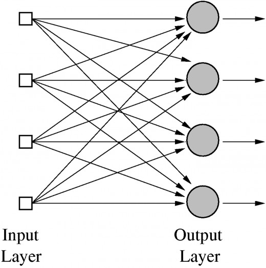
So let's say we want to build a neural net with an input size \(n_{in}\) and an output size \(n_{out}\). We then must have \(n_{out}\) neurons. Each one of our neurons then has \(n_{in}\) inputs, so it must have as many weights. If we consider the neuron number \(i\) we can call this weights \(w_{1,i},\dots,w_{n_{in},i}\) and the bias of the neuron \(b_{i}\) then the output number \(i\) is

\begin{equation*} y_{i} = f \left ( \sum_{k=1}^{n_{in}} x_{k} w_{k,i} + b_{i} \right ) \end{equation*}

where \(x_{1},\dots,x_{n_{in}}\) are the coordinates of the input. There is a more compact way to write this, with a little bit of linear algebra. The big sum inside the parenthesis is just the i-th coordinate of the matrix product \(XW\) if we define the matrix \(W\) as the array of weights \((w_{i,k})\) (with \(n_{in}\) rows and \(n_{out}\) columns) and \(X\) is a vector containing the inputs (viewed as a single row). If we then note \(Y\) the vector containing the outputs and \(B\) the vector containing the biases (both have \(n_{out}\) coordinates), we can simply write

\begin{equation*} Y = f(XW + B) \end{equation*}

where \(f\) is applied to each one of the coordinates of the vector \(XW + B\).

This is the only thing a neural net does, apply a linear operation then an activation function. Except it does that many times: instead of having just one layer of neurons, we have multiple ones, each one feeding the next.

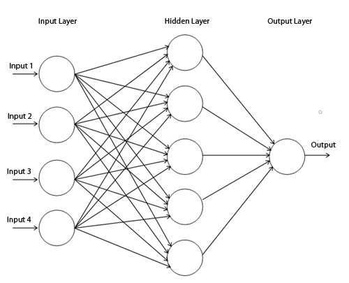
Here we have three layers, each one having its own set of weights \(W_{l}\), its vector of biases \(B_{l}\) and its activation function \(f_{l}\). The only constraint is that each vector of bias as the same number of coordinates as the number of columns of the weigh matrix, which must also be the number of rows of the next weight matrix.

If we have an input \(X\), we compute the output by going through each layer, one after the other:

\begin{equation*} \left \{ \begin{array}{l} X_{0} = X \\ X_{1} = f_{0}(X_{0}W_{1} + B_{1}) \\ X_{2} = f_{1}(X_{1}W_{2} + B_{2}) \\ \vdots \\ X_{L} = f_{L}(X_{L-1}W_{L} + B_{L}) \end{array} \right . \end{equation*}

where \(L\) is the number of layers. This is when we see why each activation function must be non-linear. If one (say \(f_{0}\)) was linear, the operations going from \(X_{0}\) to \(X_{1}W_{2} + B_{2}\) would all be linear, so they could be summarized in to

\begin{equation*} X_{1}W_{2} + B_{2} = X_{0}W'_{1} + B'_{1} \end{equation*}

and there wouldn't be any need to have that initial first layer.

Training

Now that we know what a neural net is, we can study how we can teach him to solve a particular problem. All the weights and the biases of the neural net we saw before (that are called the parameters of our model) are initialized at random, so initially, the output the neural net will compute has nothing to do with what we would expect. It's through a process called training that we will make our model better.

To do this, we need a set of labeled data, which is a collection of inputs where we know the desired output, for instance, in an image classification problem, pictures that have been classified for us. We can then evaluate how badly our model is doing by computing all the outputs and comparing them to the theoretical ones. To give a value to this, we use an error function.

An error function that is often used is called MSE for Mean Squared Errors. If \(Y\) is the output we computed and \(Z\) the one we should have found, one way to see how far away \(Y\) is from \(Z\) is to take the mean of the errors between each coordinate \(y_{i}\) and \(z_{i}\). This error can be represented by \((z_{i}-y_{i})^{2}\). The square is to get rid of the negatives (an error of -4 is as bas as an error of 4). If \(Y\) and \(Z\) are of size \(n_{out}\), this can be written

\begin{equation*} \hbox{MSE}(Y,Z) = \frac{1}{n_{out}} \sum_{i=1}^{n_{out}} (z_{i}-y_{i})^{2}. \end{equation*}

And then we can define the total loss by taking the mean of the loss on all our data. If we have \(N\) inputs \(X_{1},\dots,X_{N}\) that are labeled \(Z_{1},\dots,Z_{N}\) (the theoretical outputs we are supposed to get), by computing what the network returns when you feed it the \(X_{i}\) and naming this as \(Y_{i}\) we then have

\begin{equation*} \hbox{loss} = \frac{1}{N} \sum_{k=1}^{N} \hbox{MSE}(Y_{k},Z_{k}) \end{equation*}

Any kind of function could be used for the loss, as long as it's always positive (you don't want to subtract things from previous losses), that it only vanishes at zero, and that it's easy to differentiate. The total loss is always taken by averaging the loss on all the samples of the dataset.

Since the network's parameters are initialized at random, this loss will be pretty bad at the beginning. Training is a process during which the computer will compute this loss, analyze why it's so bad, and try to do a little bit better the next time. More specifically, we will try to determine a new set of parameters (all the weights and the biases) that will give us a slightly better loss. Then by repeating this over and over again, we should find the set of parameters that minimize this loss.

The exciting thing with neural networks, is that even if they learn on a specific dataset, they tend to generalize pretty well (and there's a bunch of techniques we can use to make sure the model doesn't overfit to the training data). In image recognition for instance, those kinds of models can have better accuracy than humans do.

To minimize this loss, we use an algorithm called SGD for Stochastic Gradient Descent. The idea is fairly simple: if you're in the mountains and looking for the point that is at the lowest altitude, you just take a step down, and a step down, and so forth until you reach that particular spot. This is going to be exactly the same for our neural net and its loss. To minimize that function, we will take a little step down.

This function loss depends of a certain amount of parameters \(p_{1},\dots,p_{t}\) (all the weights and all the biases). Now, with just a little bit of math, we know that the way down for a function of \(t\) variables (which is the direction where it's steeper) is given by the opposite of the gradient. This is the vector

\begin{equation*} \overrightarrow{\hbox{grad}}(\hbox{loss}) = \left ( \frac{\partial \hbox{loss}}{\partial p_{1}}, \dots, \frac{\partial \hbox{loss}}{\partial p_{t}} \right ) \end{equation*}

To update our parameters, which just have to take a step along the opposite of the gradients, which means subtract to the vector \((p_{1},\dots,p_{t})\) a little bit multiplied by this gradient vector. How much? That's the question that has been driving crazy a lot of data scientists, and we will give an answer in another article. This little bit is called the learning rate, and if we note it \(\hbox{lr}\) we can update our parameters with the formulas:

\begin{equation*} \hbox{new } p_{i} = \hbox{old } p_{i} - \hbox{lr} \times \frac{\partial \hbox{loss}}{\partial p_{i}}. \end{equation*}

By doing this, we know that the loss, the next time we compute all the outputs of all our data, is going to be better (the only exception would be if we chose a too high learning rate, which would make us miss the spot where our function was lowest, but we'll get back to this later). So by repeating this step over and over again, we will eventually get to a minimum of our loss function, and a very good model.

This explains the Gradient Descent in SGD but not the Stochastic part. The random part appears by necessity: very often our training dataset has a lot of labeled inputs. It can be as big as a million images. That's why, for a step of gradient descent, we don't compute the total loss, but rather the loss on a smaller sample called a mini-batch. If we choose to take the sample \((X_{k_{1}},Z_{k_{1}}),\dots,(X_{k_{mb}},Z_{k_{mb}})\) the loss on this mini-batch will just be:

\begin{equation*} \hbox{loss}' = \frac{1}{mb} \sum_{q=1}^{mb} \hbox{MSE}(Y_{k_{q}},Z_{k_{q}}) \end{equation*}

The idea is that this new loss will have a gradient that is close to the gradient of the real loss (since we're averaging on a mini-batch and not just taking one sample) but with fewer computation time. In practice, to make sure we still see all of the data, we don't overlap the mini-batches, taking different parts of our training set each time we randomly pick a mini-batch, and updating all the parameters of our network each time, up until we have seen all the inputs once. This whole process is called an epoch.

We can then run as many epochs as we want (or as we have time to), as long as the learning rate is low enough, the neural network should progress and become better each time. The gradient may seem a bit complicated to evaluate, but it can be computed exactly by using the chain rule, going backward from the end (compute the derivatives of the loss function with respects to the obtained outputs), through each layer, up until the beginning.

That is all the general theory behind a neural network. I will dig more into the details in further articles to explain the different layers we can find, the little tweaks we can add to SGD to make it train faster, how to set the learning rate and how to compute those gradients. We'll see how to code simple and more complex examples of neural networks in pytorch, but you can already jump a bit ahead and look at the first video of the deep-learning course of fast.ai, and train in a few minutes a neural net recognizing cats from dogs with 99% accuracy.