How Do You Find A Good Learning Rate
Posted on Tue 20 March 2018 in Basics
The theory
How do you decide on a learning rate? If it's too slow, your neural net is going to take forever to learn (try to use \(10^{-5}\) instead of \(10^{-2}\) in the previous article for instance). But if it's too high, each step you take will go over the minimum and you'll never get to an acceptable loss. Worse, a high learning rate could lead you to an increasing loss until it reaches nan.
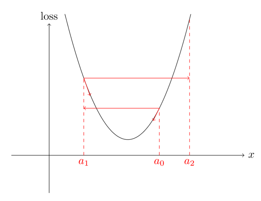
Why is that? If your gradients are really high, then a high learning rate is going to take you to a spot that's so far away from the minimum you will probably be worse than before in terms of loss. Even on something as simple as a parabola, see how a high learning rate quickly gets you further and further away from the minima.
So we have to pick exactly the right value, not too high and not too low. For a long time, it's been a game of try and see, but in this article another approach is presented. Over an epoch begin your SGD with a very low learning rate (like \(10^{-8}\)) but change it (by multiplying it by a certain factor for instance) at each mini-batch until it reaches a very high value (like 1 or 10). Record the loss each time at each iteration and once you're finished, plot those losses against the learning rate. You'll find something like this:
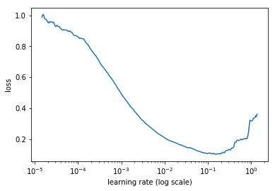
The loss decreases at the beginning, then it stops and it goes back increasing, usually extremely quickly. That's because with very low learning rates, we get better and better, especially since we increase them. Then comes a point where we reach a value that's too high and the phenomenon shown before happens. Looking at this graph, what is the best learning rate to choose? Not the one corresponding to the minimum.
Why? Well the learning rate that corresponds to the minimum value is already a bit too high, since we are at the edge between improving and getting all over the place. We want to go one order of magnitude before, a value that's still aggressive (so that we train quickly) but still on the safe side from an explosion. In the example described by the picture above, for instance, we don't want to pick \(10^{-1}\) but rather \(10^{-2}\).
This method can be applied on top of every variant of SGD, and any kind of network. We just have to go through one epoch (usually less) and record the values of our loss to get the data for our plot.
In practice
How do we code this? Well it's pretty simple when we use the fastai library. As detailed in the first lesson, if we have built a learner object for our model, we just have to type
learner.lr_find()
learner.sched.plot()
and we'll get a picture very similar as then one above. Let's do it ourselves though, to be sure we have understood everything there is behind the scenes. It's going to be pretty easy since we just have to adapt the training loop seen in that article there is just a few tweaks.
The first one is that we won't really plot the loss of each mini-batch, but some smoother version of it. If we tried to plot the raw loss, we would end up with a graph like this one:
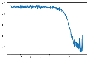
Even if we can see a global trend (and that's because I truncated the part where it goes up to infinity on the right), it's not as clear as the previous graph. To smooth those losses we will take their exponentially weighed averages. It sounds far more complicated that it is and if you're familiar with the momentum variant of SGD it's exactly the same. At each step where we get a loss, we define this average loss by
where \(\beta\) is a parameter we get to pick between 0 and 1. This way the average losses will reduce the noise and give us a smoother graph where we'll definitely be able to see the trend. This also also explains why we are too late when we reach the minimum in our first curve: this averaged loss will stay low when our losses start to explode, and it'll take a bit of time before it starts to really increase.
If you don't see the exponentially weighed behind this average, it's because it's hidden in our recursive formula. If our losses are \(l_{0},\dots,l_{n}\) then the exponentially weighed loss at a given index \(i\) is
so the weights are all powers of \(\beta\). If remember the formula giving the sum of a geometric sequence, the sum of our weights is
so to really be an average, we have to divide our average loss by this factor. In the end, the loss we will plot is
This doesn't really change a thing when \(i\) is big, because \(\beta^{i+1}\) will be very close to 0. But for the first values of \(i\), it insures we get better results. This is called the bias-corrected version of our average.
The next thing we will change in our training loop is that we probably won't need to do one whole epoch: if the loss is starting to explode, we probably don't want to continue. The criteria that's implemented in the fastai library and that seems to work pretty well is:
Lastly, we need just a tiny bit of math to figure out by how much to multiply our learning rate at each step. If we begin with a learning rate of \(\hbox{lr}_{0}\) and multiply it at each step by \(q\) then at the \(i\)-th step, our learning rate will be
Now, we want to figure out \(q\) knowing \(\hbox{lr}_{0}\) and \(\hbox{lr}_{N-1}\) (the final value after \(N\) steps) so we isolate it:
Why go through this trouble and not just take learning rates by regularly splitting the interval between our initial value and our final value? We have to remember we will plot the loss against the logs of the learning rates at the end, and if we take the log of our \(\hbox{lr}_{i}\) we have
which corresponds to regularly splitting the interval between our initial value and our final value... but on a log scale! That way we're sure to have evenly spaced points on our curve, whereas by taking
we would have had all the points concentrated near the end (since \(\hbox{lr}_{N-1}\) is much bigger than \(\hbox{lr}_{0}\)).
With all of this, we're ready to alter our previous training loop. This all supposes that you've got a neural net defined (in the variable called net), a data loader called trn_loader, an optimizer and a loss function (called criterion).
def find_lr(init_value = 1e-8, final_value=10., beta = 0.98):
    num = len(trn_loader)-1
    mult = (final_value / init_value) ** (1/num)
    lr = init_value
    optimizer.param_groups[0]['lr'] = lr
    avg_loss = 0.
    best_loss = 0.
    batch_num = 0
    losses = []
    log_lrs = []
    for data in trn_loader:
        batch_num += 1
        #As before, get the loss for this mini-batch of inputs/outputs
        inputs,labels = data
        inputs, labels = Variable(inputs), Variable(labels)
        optimizer.zero_grad()
        outputs = net(inputs)
        loss = criterion(outputs, labels)
        #Compute the smoothed loss
        avg_loss = beta * avg_loss + (1-beta) *loss.data[0]
        smoothed_loss = avg_loss / (1 - beta**batch_num)
        #Stop if the loss is exploding
        if batch_num > 1 and smoothed_loss > 4 * best_loss:
            return log_lrs, losses
        #Record the best loss
        if smoothed_loss < best_loss or batch_num==1:
            best_loss = smoothed_loss
        #Store the values
        losses.append(smoothed_loss)
        log_lrs.append(math.log10(lr))
        #Do the SGD step
        loss.backward()
        optimizer.step()
        #Update the lr for the next step
        lr *= mult
        optimizer.param_groups[0]['lr'] = lr
    return log_lrs, losses
Note that the learning rate is found into the dictionary stored in optimizer.param_groups. If we go back to our notebook with the MNIST data set, we can then define our neural net, an optimizer and the loss function.
net = SimpleNeuralNet(28*28,100,10)
optimizer = optim.SGD(net.parameters(),lr=1e-1)
criterion = F.nll_loss
And after this we can call this function to find our learning rate and plot the results.
logs,losses = find_lr()
plt.plot(logs[10:-5],losses[10:-5])
The skip of the first 10 values and the last 5 is another thing that the fastai library does by default, to remove the initial and final high losses and focus on the interesting parts of the graph. I added all of this at the end of the previous notebook, and you can find it here.
This code modifies the neural net and its optimizer, so we have to be careful to reinitialize those after doing this, to the best value we can. An amelioration to the code would be to save it then reload the initial state when we're done (which is what the fastai library does).