Convolution in depth
Posted on Thu 05 April 2018 in Basics
Since AlexNet won the ImageNet competition in 2012, linear layers have been progressively replaced by convolutional ones in neural networks trained to perform a task related to image recognition. Let's see what those layers do and how to implement them from scratch.
What is convolution?
The idea behind convolution is the use of image kernels. A kernel is a small matrix (usually of size 3 by 3) used to apply effect to an image (like sharpening, blurring...). This is best shown on this super cool page where you can actually see the direct effect on any image you like.
The core idea is that an image is just a bunch of numbers. Its representation in a computer is an array of size width by heights pixels, and each pixel is associated to three float values ranging from 0 to 1 (or integers going from 0 to 255). This three numbers represent the red-ness, green-ness and blue-ness of said pixel, the combination of the three capturing its color. A fourth channel can be added to represent the transparency of the pixel but we won't focus on that.
If the image is black and white, a single value can be use per pixel, with 0 meaning black and 1 (or 255) meaning white. Let's begin with this for the explanation. The convolution of our image by a given kernel of a given size is obtained by putting the kernel in front of every area of the picture, like a sliding window, to then do the element-wise product of the numbers in our kernel by the ones in the picture it overlaps and summing all of these, like in this picture:
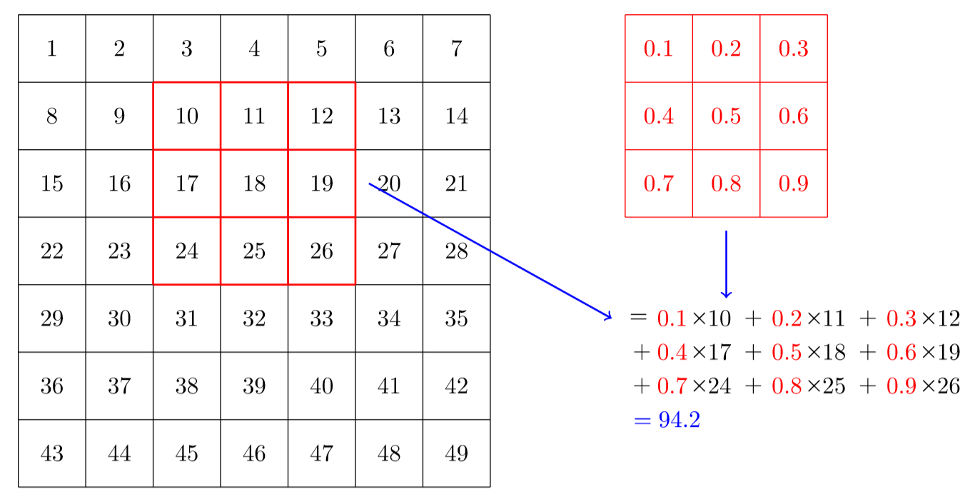
Then we repeat the process by moving the kernel on every possible area of the picture.
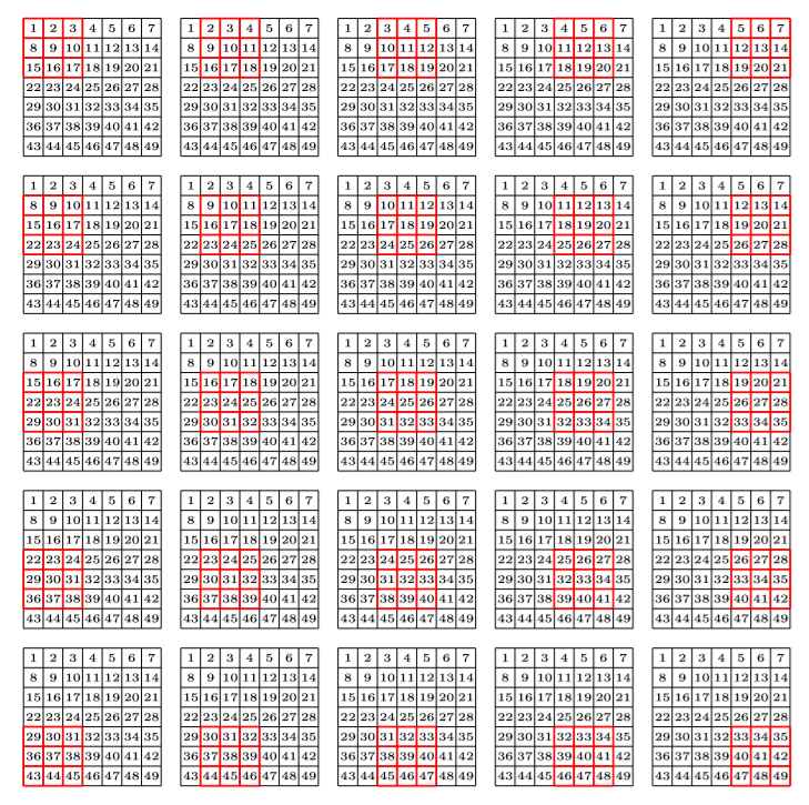
As shown on this page mentioned earlier, by doing this on all the areas of our picture, sliding the kernel in all the possible positions, it will give another array of number that we can also interpret as a picture, and depending on the values inside of our kernel, this will apply different effects on the original image. The process is shown on this video
The idea behind a convolutional layer in a neural net is then to initialize the weights of kernels like the one we just saw at random, then use SGD to find the best possible parameters. It's possible to do this since the operation we are doing withour sliding window looks like
with the \(w_{i,j}\) being the weights in our kernel and the \(x_{i,j}\) being the values of our pixels. We can even decide to add a bias to have exactly the same transformation as a linear layer, the only difference being that the weights of a given kernel are the same and applied to the whole picture.
By stacking several convolutional layers one on top of the other, the hope is to get a neural network that captures the information we want on our image.
Stride and padding
Before we implement a convolutional layer in python, there is a few additional tweaks we can add. Padding consists in adding a few pixels on each (or a few) side of the picture with a zero value. By doing this, we can have an output that has exactly the same dimension is the output. For instance if we have an 7 by 7 image with a 3 by 3 kernel like in the picture before, you can put the sliding window on 5 (7 - 3 + 1) different position in width and height, so you get a 5 by 5 output. Adding a border of width one pixel all around the picture will change the original image into a 9 by 9 picture and make an output of size 7 by 7.
A stride in convolution is just like a by in a for loop: instead of going through every window one after the other, we skip a given amount each time. Here is the result of a convolution with a padding of one and a stride of two:
In the end, if our picture as \(n_{1}\) rows and \(n_{2}\) columns, our kernel \(k_{1}\) rows and \(k_{2}\) columns, with a padding of \(p\) and a stride of \(s\), the dimension of the new picture is
Why is that? Well for the width dimension, our picture has a size of \(n_{1} + 2*p\) since we added \(p\) pixels on each side. We begin in position 0 and the maximum index at the far right is \(n_{1} + 2*p-k_{1}\). Since we move by steps of length \(s\), the last position we reach is \(\hbox{nb} s\) where \(\hbox{nb}\) is the highest number satisfying
which gives us
Then from 0 to \(\hbox{nb}\), there is \(\hbox{nb}+1\) integer, which is how we find the width of the output. It's the same reasoning for the height.
More channels
We gave the example of a black and white picture, but when we have an image with colors, there are three different channels. This means that our filter will need the same number of channels. In the previous example, instead of having just one 3 by 3 kernel, we'll have three. One for the red values of each pixel, one for the green values of each pixel and one of their blue values. So our filter is 3 channels by 3 by 3. We place the red part in front of the red channel of our picture, the green part in front of the green channel and the blue part in front of the blue channel, each time at exactly the same place like this.
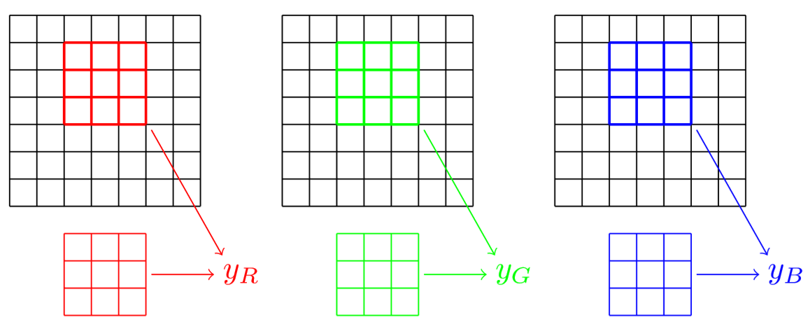
The results of those three intermediate convolutions \(y_{R}\), \(y_{G}\) and \(y_{B}\) are computed as before, and we sum them to get our final activation. It's get a bit more complicated because this is just one kernel. To make a full layer, we will consider several of them and use them all on all the possible places of our picture, with padding and stride if applicable.
Before the layer we had a picture with 3 channels, width \(n_{1}\) and height \(n_{2}\), after, we have another representation of that image with as many channels as we decided to take filters (let's say \(nb_{F}\)), width \(nb_{1}\) and height \(nb_{2}\) (those two numbers being calculated with the formula above). If the initial channels represented the red-ness, green-ness, blue-ness of a pixel, the new ones will represent things like horizontal-ness or bluri-ness of a given area.
When we stack this into a new convolutional layer (with kernels of size \(nb_{F}\) by 3 by 3) it becomes harder to figure what the channels we obtain represent, but we don't necessarily need to understand their meaning. What's important is that the neural net will find a set of weights (via SGD) that helps it get the key informations it needs to eventually perform the task it was given (like identifying the digit in the picture, or classifying it between cat and dog).
Let's code this!
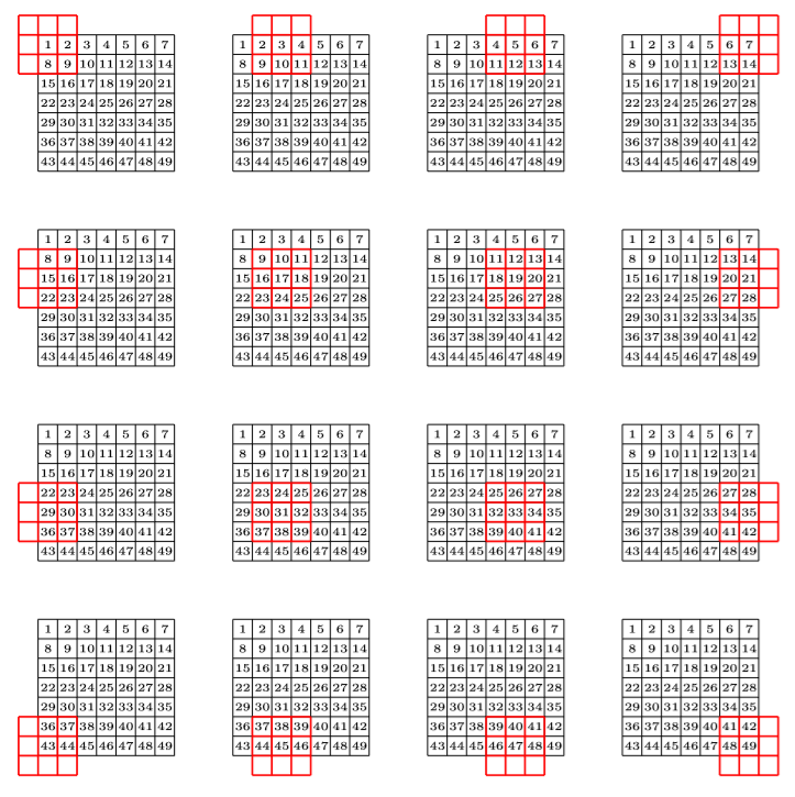
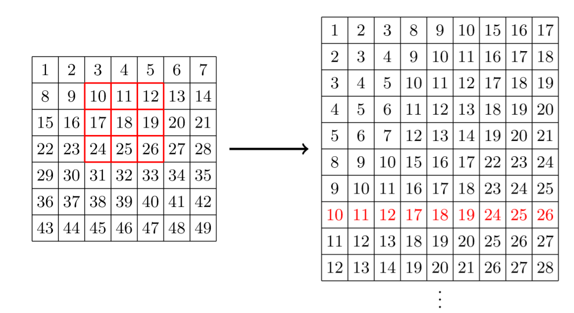
Coding this in numpy is not the easiest thing so feel free to skip this part. It does provide good practice on vectorization and broadcasting though. We won't code the convolution as a loop since it would be very inefficient when with have to do it on a whole mini-batch. Instead, we will vectorize our picture so that the convolution operation just becomes a matrix product (which it is in essence, since it's a linear operation). This means taking each small window our kernel will look at and writing the number we see in a row.
Taking back the 7 by 7 matrix before with a 3 by 3 kernel, it will change it like this (red window is written in red in our vector).
If we note \(\hbox{vec}(x)\) the vectorization of \(x\), and if we write our weights in a column \(W\) (in the same order as with our windows), then the result of our convolution is just
If we want to have the result of the convolution with all our filters at once, we just have to concatenate the corresponding columns into a matrix (that we will still note \(W\)) and the same matrix product will give us all the results at the same time.
That's for one channel, but what happens when we have more? We can just concatenate the vectorization for each channel in a very big \(\hbox{vec}(x)\), and put all the weights in the same order in a column of \(W\).
Each row in this table represent a particular 3 by 3 window, which has 9 coordinates in each of the channels (red, green and blue), which is why they have 27 coordinates. There are 25 possibilities to align a window in front of our picture, which is why there 25 rows.
The last thing we can do is define a bias for each of our kernel, and if we write them in a table named \(B\), the result of our convolution is
where \(B\) has as many columns as \(W\) (\(nb_{F}\)) and his coordinates are broadcasted over the row (e.g. repeated as many times as necessary to make \(B\) the same size as the matrix before.
Last part is to reshape the result \(y_{1}\). Let's go back to the input \(x\). In practice, we will get a whole mini-batch of them, which gives a new dimension (three was too easy already...). So the size of \(x\) is \(m\) (for mini-batch) by \(ch\) (3 if we have the original picture) by \(n_{1}\) by \(n_{2}\). When we vectorize it, \(\hbox{vec}(x)\) has a size of \(m\) by \(nb_{1} \times nb_{2}\) (all the possibilities to put our filter in front of our image) by \(k_{1} \times k_{2} \times ch\) (where the kernel is assumed of size \(k_{1}\) by \(k_{2}\)).
Our matrix \(W\) has \(nb_{F}\) columns (the number of filters) and \(k_{1} \times k_{2} \times ch\) rows, so the product will give us a result \(y_{1}\) of size \(m\) by \(nb_{1} \times nb_{2}\) by \(nb_{F}\) (assuming we broadcast the product over the first dimension, doing it for all mini-batch). The channels should be the second dimension if we want to be consistent with how we treated \(x\) so we have to transpose the two last dimensions, and finally resize the result as \(y\), with a shape of \(m\) by \(nb_{F}\) by \(nb_{1}\) by \(nb_{2}\).
That sounds awfully complicated but as soon as we are done with the first part (vectorize the picture) the rest will be very easy.
Forward pass
Let's assume first we already have that vectorization function that I'll call arr2vec. Since it's the hardest bit, let's keep it for the end. As we saw before, there's no point in our computation where we will need the weights other than in the form of the matrix \(W\), so that's how we will store and create them. As for a linear layer, the best way to initialize them is by following a normal distribution with a standard deviation of \(\sqrt{\frac{2}{ch}}\) if \(ch\) is the number of channels of the input.
For the forward pass, we vectorize the mini-batch of inputs x, then we multiply the result by our weights and our bias. Then we have to invert the two last axis and reshape with the output size, which can be computed with the formulas above. All in all, this gives us:
class Convolution():

    def __init__(self, nc_in, nc_out, kernel_size, stride=2,padding=1):
        self.kernel_size = kernel_size
        self.weights = np.random.randn(nc_in * kernel_size[0] * kernel_size[1] ,nc_out) * np.sqrt(2/nc_in)
        self.biases = np.zeros(nc_out)
        self.stride = stride
        self.padding = padding

    def forward(self,x):
        mb, ch, n, p = x.shape
        y = np.matmul(arr2vec(x,self.kernel_size,self.stride,self.padding), self.weights) + self.biases
        y = np.transpose(y,(0,2,1))
        n1 = (n-self.kernel_size[0]+ 2 * self.padding) //self.stride + 1
        p1 = (p-self.kernel_size[1]+2 * self.padding )//self.stride + 1
        return y.reshape(mb,self.biases.shape[0],n1,p1)
The arr2vec function remains. To write it, let's go back to the previous picture:
The whole problem is to do this, once this is done, we'll just have to take the corresponding elements in our array x (instead of aligning 1,2,3, we'll need x[1],x[2],x[3]). We can note that each row in the vectorization can be deduced from the first by adding the same number everywhere. Let's forget about padding and stride to begin with and start with this first line.
Since we're in Python, indexes begin at 0. Then we just want the numbers \(j+i*n_{2}\) where \(j\) goes from 0 to \(k_{1}\), \(i\) goes from 0 to \(k_{2}\) and \(n_{2}\) is the number of columns. Those will form the grid of our kernel. Then we have to determine all the possible start indexes, which correspond to the points with coordinates \((i,j)\) where \(i\) can vary from 0 to \(n_{1} - k_{1}\) and \(j\) can vary from 0 to \(n_{2} - k_{2}\). For a given couple \((i,j)\), the index associated is \(j + i * n_{2}\). This gives us:
grid = np.array([j + n2*i for i in range(k1) for j in range(k2)])
start_idx = np.array([j + n2*i for i in range(n1-k1+1) for j in range(n2-k2+1) ])
Why the np.array? Well once we have done this, we basically want the array built by getting grid + any element in start_idx, which is very easy to do with broadcasting. Our vectorized array of indexes is:
grid[None,:] + start_idx[:,None]
Let's add a bit more complexity now. This is all we need for one channel, but we will actually get \(ch\) of them. Our start indexes won't change since they are the same for all the channels, but our grid must include more element. Specifically, we need to duplicate the grid \(ch\) times, adding \(n_{1} \times n_{2}\) each time we do. This is done by
grid = np.array([j + n2*i + n1 * n2 * k for k in range(0,ch) for i in range(k1) for j in range(k2)])
Now for the stride and padding. Padding is adding 0 on the sides so we can begin by this.
y = np.zeros((mb,ch,n1+2*padding,n2+2*padding))
y[:,:,padding:n1+padding,padding:n2+padding] = x
This doesn't change our grid much, we will just have to adapt the sizes of our picture (now \(n_{1} + 2p\) by \(n_{2} + 2p\)). The start indexes will change slightly: the upper bound for the indexes \(i\) and \(j\) are now \(n_{1} +2p - k_{1}\) and \(n_{2} + 2p - k_{2}\). Stride only adds one thing: we loop with a step.
start_idx = np.array([j + (n2+2*padding)*i for i in range(0,n1-k1+1+2*padding,stride) for j in range(0,n2-k2+1+2*padding,stride) ])
grid = np.array([j + (n2+2*padding)*i + (n1+2*padding) * (n2+2*padding) * k for k in range(0,ch) for i in range(k1) for j in range(k2)])
to_take = start_idx[:,None] + grid[None,:]
The last step is to do this for each mini-batch. Again, this will easily be done with a bit of broadcasting:
batch = np.array(range(0,mb)) * ch * (n1+2*padding) * (n2+2*padding)
batch[:,None,None] + to_take[None,:,:]
This final arrays has exactly the same shape as our desired output, and contains all the indexes we have to take in our array y. We just have to use the function numpy.take to select the corresponding elements in y.
def arr2vec(x, kernel_size, stride=1,padding=0):
    k1,k2 = kernel_size
    mb, ch, n1, n2 = x.shape
    y = np.zeros((mb,ch,n1+2*padding,n2+2*padding))
    y[:,:,padding:n1+padding,padding:n2+padding] = x
    start_idx = np.array([j + (n2+2*padding)*i for i in range(0,n1-k1+1+2*padding,stride) for j in range(0,n2-k2+1+2*padding,stride) ])
    grid = np.array([j + (n2+2*padding)*i + (n1+2*padding) * (n2+2*padding) * k for k in range(0,ch) for i in range(k1) for j in range(k2)])
    to_take = start_idx[:,None] + grid[None,:]
    batch = np.array(range(0,mb)) * ch * (n1+2*padding) * (n2+2*padding)
    return y.take(batch[:,None,None] + to_take[None,:,:])
Back propagation
If you've made it this far, there is just one last step to have completely understood a convolutional layer: we need to compute the gradients of the loss with respect to the weights, the biases and the inputs, being given the gradients of the loss with respect to the outputs.
At heart, a convolutional layer is just a certain type of linear layer, so the formulas we had seen for the back-propagation through a linear layer will be useful here too. There is just a bit of reshaping, transposing, and... sadly... going back from a vector to an array. But let's keep this for last, since it'll be the worst.
When we receive our gradient in a variable grads, they will have the same shape as our final output y, so \(m\) by \(nb_{F}\) by \(nb_{1}\) by \(nb_{2}\). To go back to \(y_{1}\), we have to reshape our gradients as \(m\) by \(nb_{F}\) by \(nb_{1} \times nb_{2}\) then invert the two alst coordinates. This will give us grad1.
The operation we did at this stage is
so we already know the gradients of the loss with respect to \(\hbox{vec}(x)\) is \({}^{t} W \hbox{grad}_{1}\) (like in this article) Following the same lead, the gradients of the loss with respect to the biases should be in grad1, but this time this array has one dimension too many. That's because each bias is used for all the activations (whereas before they were only used once). We will have to sum the gradients over all the activations they appear (that's the second dimension of grad1), then take the mean over the mini-batch (which is the first dimension).
Why the sum? It comes from the chain rule. Since a given bias \(b\) is used to compute \(z_{1},\dots,z_{N}\) (where \(N = nb_{1} \times nb_{2}\)) we have
It'll be the same for the weights: for a given weight \(w_{i,j}\), we have to compute all the vec(x)[:,:,i] * grad1[:,:,j] then take the sum over the second axis, and take the mean over the first axis.
Then, we have to reshape the gradient of the loss with respect to \(\hbox{vec}(x)\) with the initial shape of x, which will need another function called vec2arr that we will code last. With all of this, we can write the full Convolution class:
class Convolution():

    def __init__(self, nc_in, nc_out, kernel_size, stride=2,padding=1):
        self.kernel_size = kernel_size
        self.weights = np.random.randn(nc_in * kernel_size[0] * kernel_size[1] ,nc_out) * np.sqrt(2/nc_in)
        self.biases = np.zeros(nc_out)
        self.stride = stride
        self.padding = padding

    def forward(self,x):
        mb, ch, n, p = x.shape
        self.old_size = (n,p)
        self.old_x = arr2vec(x,self.kernel_size,self.stride,self.padding)
        y = np.matmul(self.old_x, self.weights) + self.biases
        y = np.transpose(y,(0,2,1))
        n1 = (n-self.kernel_size[0]+ 2 * self.padding) //self.stride + 1
        p1 = (p-self.kernel_size[1]+2 * self.padding )//self.stride + 1
        return y.reshape(mb,self.biases.shape[0],n1,p1)

    def backward(self,grad):
        mb, ch_out, n1, p1 = grad.shape
        grad = np.transpose(grad.reshape(mb,ch_out,n1*p1),(0,2,1))
        self.grad_b = grad.sum(axis=1).mean(axis=0)
        self.grad_w = (np.matmul(self.old_x[:,:,:,None],grad[:,:,None,:])).sum(axis=1).mean(axis=0)
        new_grad = np.matmul(grad,self.weights.transpose())
        return vec2arr(new_grad, self.kernel_size, self.old_size, self.stride, self.padding)
The last function takes a vectorized input and has to compute an array associated to it by reversing what arr2vec is doing. It's not just repositioning elements: in the earlier example, 3 was present three times. The elements on those positions must be summed (the chain rule again) and the result placed in the position where 3 was in the initial array.
So that's what we have to do: for each element on our initial array, we have to locate all the spots the arr2vec function put them in, sum the elements we get, and put that in our result array. To use vectorization, we will create a big array of numbers, with as many row as as in our input, so \(N = m \times ch \times n_{1} \times n_{2}\) and as many columns as necessary. On each row, we will have the positions of where the arr2vec function would have placed that element, so we will just have to take the sum over the second axis and reshape at the end.
First, let's check how many windows could have passed over the element with coordinates \((i,j)\). That's all the windows that started at \((i-k1i,j-k2j)\) where \(k1i\) can go from 0 to \(k_{1}-1\) and \(k2j\) can go from 0 to \(k_{2}-1\). Of course, this will sometimes give us negatives coordinates, or coordinates of window that go to far on the right or the bottom of the picture. We'll deal with those with a mask, but first, let's compute them all.
idx = np.array([[[i-k1i, j-k2j] for k1i in range(k1) for k2j in range(k2)] for i in range(n) for j in range(p)])
in_bounds = (idx[:,:,0] >= -padding) * (idx[:,:,0] <= n-k1+padding)
in_bound *= (idx[:,:,1] >= -padding) * (idx[:,:,1] <= p-k2+padding)
The second array is a boolean array that checks that the corners of our windows are inside the picture, taking the padding into account. Another mask we will need is to take the stride into account: some of those windows aren't considered if we have a stride different from one.
in_strides = ((idx[:,:,0]+padding)%stride==0) * ((idx[:,:,1]+padding)%stride==0)
Now we can just convert the couples into indexes and our channel dimension at the bottom.
to_take = np.concatenate([idx[:,:,0] * k2 + idx[:,:,1] + k1*k2*c for c in range(ch)], axis=0)
At this stage, we read on a line (when it's in bound and in-stride) the indexes of the elements to pick in each column. For this to correspond to the indexes of the element in the array, we have to add to each column a multiple of the number of columns in our input (which I called ftrs).
to_take = to_take + np.array([ftrs * i for i in range(k1*k2)])
to_take = np.concatenate([to_take + md*ftrs*m for m in range(mb)], axis=0)
Then we add all the mini-batches over the same dimension. Last thing we have to do is to expand our mask to make it the same size.
in_bounds = np.tile(in_bounds * in_strides,(ch * mb,1))
and we're ready to take our inputs and sum them!
def vec2arr(x, kernel_size, old_shape, stride=1,padding=0):
    k1,k2 = kernel_size
    n,p = old_shape
    mb, md, ftrs = x.shape
    ch = ftrs // (k1*k2)
    idx = np.array([[[i-k1i, j-k2j] for k1i in range(k1) for k2j in range(k2)] for i in range(n) for j in range(p)])
    in_bounds = (idx[:,:,0] >= -padding) * (idx[:,:,0] <= n-k1+padding)
    in_bounds *= (idx[:,:,1] >= -padding) * (idx[:,:,1] <= p-k2+padding)
    in_strides = ((idx[:,:,0]+padding)%stride==0) * ((idx[:,:,1]+padding)%stride==0)
    to_take = np.concatenate([idx[:,:,0] * k2 + idx[:,:,1] + k1*k2*c for c in range(ch)], axis=0)
    to_take = to_take + np.array([ftrs * i for i in range(k1*k2)])
    to_take = np.concatenate([to_take + md*ftrs*m for m in range(mb)], axis=0)
    in_bounds = np.tile(in_bounds * in_strides,(ch * mb,1))
    return np.where(in_bounds, np.take(x,to_take), 0).sum(axis=1).reshape(mb,ch,n,p)