Recurrent Neural Network

The general principle

A Recurrent Neural Network basically looks like this:

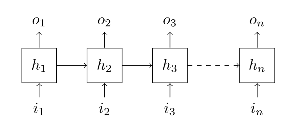
From our first input \(i_{1}\), we compute a first hidden state \(h_{1}\). How? Like a neural net does, with a linear layer. From this hidden state, we compute an output \(o_{1}\), again with a linear layer. This part is no different than a regular neural net with one hidden layer. What changes is that when we have our second input \(i_{2}\), we do use the same linear layer as \(i_{1}\) to compute the arrow going from \(i_{2}\) to \(h_{2}\) but we had something: the previous hidden state \(h_{1}\) goes through a linear layer of its own and we merge the two results to get \(h_{2}\), then \(o_{2}\) is calculated from \(h_{2}\) the same way \(o_{1}\) was from \(h_{1}\).

Then we continue the same way up until the end. There may be many arrows in that figure, but there's only three linear layers in this neural net, they are just repeated several times. Specifically, we need a layer \(L_{ih}\), that goes from input to hidden, a layer \(L_{hh}\) that goes from hidden to hidden, and a layer \(L_{ho}\) that goes from the hidden state to the output. Following the same notations, we have weight matrices \(W_{ih}\), \(W_{hh}\) and \(W_{ho}\), bias vectors \(b_{ih}\), \(b_{hh}\) and \(b_{ho}\). If we note \(n_{in}\) the size of the input, \(n_{hid}\) the size of the hidden state and \(n_{out}\) the size of the output, naturally we have the following sizes:

and the following equations to compute the next stage from the previous one:

To complete these, the first value of hidden state \(h_{0}\) is assumed to be zeros. Note that the way we merged the two arrows here is by summing them, but after applying the linearity. An equivalent way to see this is that we concatenated \(i_{k}\) and \(h_{k-1}\) then applied a weight matrix of size \((n_{in}+n_{hid}) \times n_{hid}\).

The two biases \(b_{ih}\) and \(b_{hh}\) are redundant, so we could only use one of them. The non-linearity inside a RNN is often tanh, because it has the advantage of spitting values between -1 and 1; a ReLU would allow for values to grow larger and larger as we apply the same linear unit every time, giving a more unstable model, and a sigmoid wouldn't give us any negatives. The non-linearity that goes to the output \(f\) can vary depending on our needs.

How to use them

A classical use for RNNs is to try to predict the next character (or word) in a text, being given the previous ones. Both problems are the same, the only difference is the size of our vocabulary: for a character-level model, we would have something between 26 and a few hundreds characters (if we want to have all the special ones, lower and upper cases). At a word-level, the model will easily have a size in the tens (if not hundreds) of thousands.

In both cases, the first step will be to split the text into tokens, which will be the characters or the words composing it (in the second case, we should actually be smarter than just taking the words, but this would be a subject for another article). Those tokens are then numericalized from 1 to n, the size of our vocabulary. We can a few extra tokens like <bos> (for beginning of stream), <eos> (end of stream) or <unk> (unknown, very useful when working at a word level: there's no use keeping the words that are barely present in our corpus since the model probably won't learn anything about them, so we can replace them all by <unk>).

Having done that, we're almost ready to feed text to a RNN. The last step is to transform those numbers that compose our texts into vectors that can pass through a neural net. When dealing at a character level, we often one-hot encode those numbers, wich means transforming i into the vector of size n with everything nil except the i-th coordinate that is 1. But doing this with words where n can be so large might not be the best idea. Instead, in those cases, we use embeddings, which is replacing each token by a vector of a given size, with random coordinates at the beginning, but that the network will then learn to make better.

We'll go into the specifics of this in another article. For now let's just see how to implement a basic RNN. The model in itself is very easily coded in pytorch, since it's a dynamical language, we can just do a for loop in the forward pass. There's a trick for the initialization: the matrix \(W_{hh}\) should be the identity matrix at the beginning and not a random one. It makes sense when we think it will be applied a lot of times to the hidden state, and not changing it at the beginning seems like a good idea. Of course, with SGD, it won't stay very long as an identity matrix.

class RNN(nn.Module):

    def __init__(self, n_in, n_hid, n_out, size):
        super().__init__()
        self.wgts_ih = torch.randn(n_in,n_hid) * np.sqrt(2/n_in)
        self.wgts_hh = torch.eye(n_hid)
        self.wgts_ho = torch.randn(n_hid,n_out) * np.sqrt(2/n_out)
        self.b_ih = torch.zeros(n_hid)
        self.b_ho = torch.zeros(n_out)
        self.size, self.n_hid = size, n_hid

    def forward(self,x):
        bs = x.size(1)
        hid = torch.zeros(bs, self.n_hid)
        outs = []
        for i in range(self.size):
            hid = F.tanh(torch.mm(x[i], self.wgts_ih) + torch.mm(hid, self.wgts_hh) + self.b_ih)
            out = torch.mm(hid, self.wgts_ho) + self.b_ho
            outs.append(out.unsqueeze(0))
        return torch.cat(outs)

Note that here in the forward pass, our tensor x has three dimensions: there is the length of the sentence, the mini-batch and the size of our vocabulary. Often in RNNs, they are indexed in this order, since it allows us to easily go through each character of our sentences via x[0], x[1], ... Here we presented the output in the same way, but depending on the goal, you might want to only keep the final output. Lastly, there's no activation function for the output since it will be computed in the loss.

Now that we have seen what's inside a RNN, we can use the module of the same name in pytorch, which would just be:

myRNN = nn.RNN(n_in, n_hid)

Here we don't specify an output size since pytorch will only give us the list of hidden states. We can decide to apply the same linear layer as we did before if we need to. When we call this network on an input (of size sequence length by batch size by vocab size), we can also specify a initial hidden state (which will be zeros if we don't), then the output will be a tupe containing two things: the list of hidden states in a tensor (except the initial one) and the last hidden state.

If we want to reproduce the previous RNN, we then have to do the following:

class RNN(nn.Module):

    def __init__(self, n_in, n_hid, n_out):
        super().__init__()
                self.rnn = nn.RNN(n_in,n_hid)
        self.linear = nn.Linear(n_hid,n_out)

    def forward(self,x):
        out, hid = self.rnn(x)
        return self.linear(out)

The last linear layer will be applied on the two first dimensions of the out tensor (one for the sequence length and one for the batch size).

Let's see some results!

By training those kind of networks a very long time on large corpus of text, one can get surprising results, even if they are just character-level trained RNNs. This article shows quite a few of them.

To get a model trained on an RNN to generate text, we just have to give it a seed: since it knows how to predict the next word from the last few, it needs a beginning. In the lesson 10 of the fasta.ai <http://fast.ai> MOOK, Jeremy shows a language model pre-trained on a subset of wikipedia. It's slightly more complex than the basic RNN we just saw, using three LSTMs, but we'll get in the depth of that in another article. Once the model is loaded in his notebook, we can use it to generate predictions by implementing this function:

def what_next(seq, res_len):
    learner.model.reset()
    tok = Tokenizer().proc_text(seq)
    ids = [stoi[word] for word in tok]
    res = []
    for i in ids:
        x = V(np.array(i)).unsqueeze(0)
        preds = learner.model(x)
        val,idx = preds[0].data.max(1)
    for i in range(res_len):
        res.append(idx[0])
        x = V(idx).unsqueeze(0)
        preds = learner.model(x)
        val,idx = preds[0].data.max(1)
    return [itos[i] for i in res]

where Tokenizer is the object we use to tokenize text (the spacy tokenizer in the notebook), itos and stoi are the mapping from tokens to ids. Using this to ask the language model What is a recurrent neural network? I got this answer:

the first of these was the first of the series, the first of which was released in october of that year.
the first, " the last of the u_n ", was released on october 1,  and the second, " the last of the u_n ",
was released on november 1.

It's not perfect, obviously, but it's interesting to note that it clearly learned basic grammar, or how to use punctuation, even closing its own quotes.