Pointer cache for Language Model
Posted on Thu 26 April 2018 in Experiments
You can easily boost the performance of a language model based on RNNs by adding a pointer cache on top of it. The idea was introduce by Grave et al. in this article and their results showed how this simple technique can make your perplexity decrease by 10 points without additional training. This sounds exciting, so let's see what this is all about and implement that in pytorch with the fastai library.
The pointer cache
To understand the general idea, we have to go back to the basic of a language model built on an RNN.
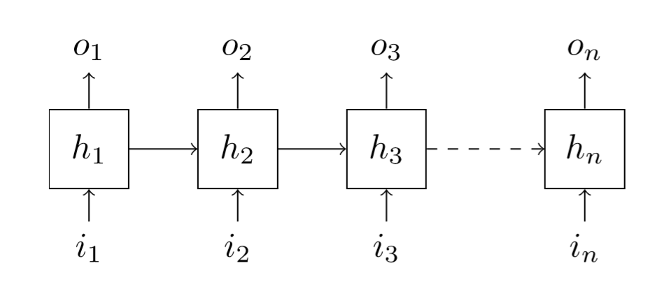
Here our inputs are words, and the outputs our predictions for the newt word to come: \(o_{1}\) should be \(i_{2}\), \(o_{2}\) should be \(i_{3}\) and so forth. What's actually inside the black box doesn't matter here, as long as we remember there is a hidden state that will be passed along the way, updated, and used to make the next predictions. When the black box is a multiple-layer RNN, what we note \(h_{t}\) is the last hidden state (the one from the final layer), which is also the one used by the decoder to compute \(o_{t}\).
Even if we had some kind of information on all the inputs \(i_{1},\dots,i_{t}\) in our hidden state to predict \(o_{t}\), it's all squeezed in the size of that hidden state, and if \(t\) is large, it has been a long time since we saw the first inputs, so all their context has probably been forgotten by now. The idea behind the pointer cache is to use again those inputs to adjust a bit the prediction \(o_{t}\).
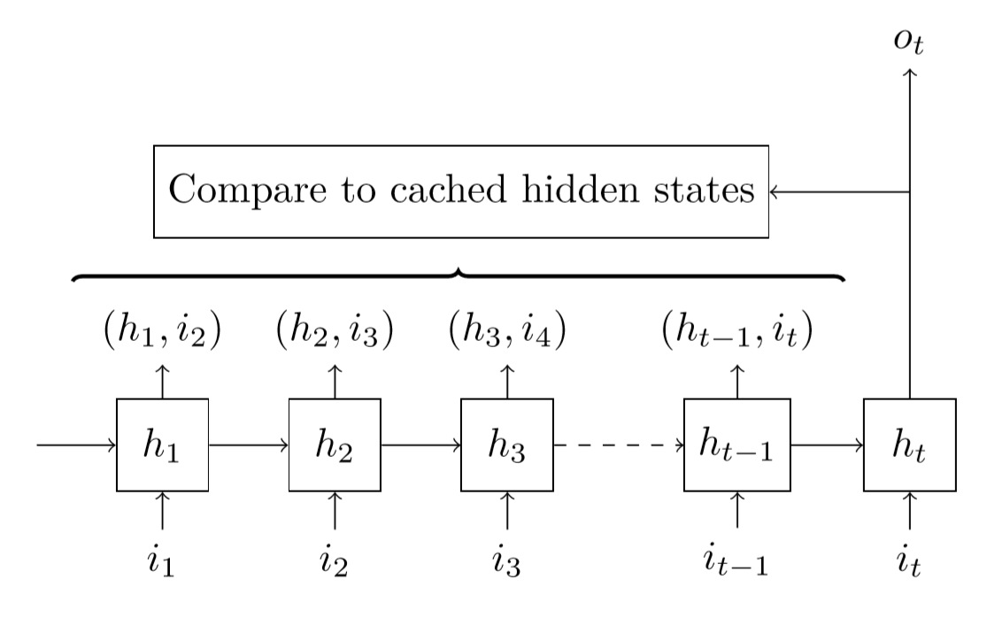
More precisely, when trying to predict \(o_{t}\), we take a look at all the previous couples \((h_{1},i_{2}),\dots,(h_{t-1},i_{t})\). The hidden state \(h_{1}\) was supposed to predict \(i_{2}\), the hidden state \(h_{2}\) was supposed to predict \(i_{3}\) and so forth. If the hidden state we have right now, \(h_{t}\) looks a lot like one of the previous hidden state \(h_{k}\), well maybe the word we are trying to predict is the same as \(h_{k}\) was supposed to, and we know that word is \(i_{k+1}\), so we should boost the probability of this word in our output \(o_{t}\).
That's the main idea behind this pointer cache technique: we really want to predict the same word as that previous hidden state, so we point at it. The cache is just that instead of looking through the history since the beginning, we only take a window of a certain length \(n\), so we look back at the \(n\) previous couples \((h_{k},i_{k+1})\).
There is just one thing to clarify: how does one code this looks a lot like thing. We simply take the dot product of \(h_{t}\) with \(h_{i}\) (which is the exact same idea as the one we saw in style transfer during the last lesson of fast.ai). The dot product will be very high if the coordinates of \(h_{t}\) and \(h_{i}\) are very high together or very low (aka very high negatives) together so it gives us a sense of how much they are similar.
From the math...
This is why in the article mentioned earlier, they come up with the formula:
It looks a lot more complicated but there is not much more than what I explained before in this line. Let's break it down in bits!
The first part is the \(p_{cache}(w | h_{1..t} x_{1..t})\). It represents a probability, more specifically a probability to have the word \(w\) while knowing \(h_{1..t} x_{1..t}\), which is a shorter way of writing \(h_{1},\dots,h_{t},x_{1},\dots,x_{t}\). The \(h_{k}\) are the hidden states and the \(x_{k}\) the inputs (what I called \(i_{k}\) because input doesn't begin with an x). So this whole thing is just a fancy way of writing what is our desired output: a vector that will contain the probabilities that the next word is \(w\) knowing all the previous inputs and hidden states.
Then there is this weird symbol \(\propto\) (which I honestly didn't know). While looking it up to type the formula, I found this very cool website where you can draw a mathematical symbol, and it will spit you its LaTeX code, and a google search of it will probably give you all the information you need to understand its meaning. Hope this trick can help you in breaking down future formulas.
Anyway, they don't use the equal sign but this proportional to because since we want a probability, we will have to have things that add up to one in the end. They don't want to bother with it for now, so this is just a way of saying: we'll give that value, and at the end, divide by the sum of all of those so we're sure it adds up to one.
Then comes a sum, going from 1 to \((t-1)\), that just means we look at all our previous hidden states. All? Not really, cause this weird 𝟙 with a double bar is an indicator function. Though more than its name, you're probably more interested in what it does. So when we have a 𝟙 like this, there is a condition written in index (here \(\{w = x_{i+1}\}\)) and the quantity is equal to 1 when the condition is true, 0 when the condition is false. So we're not summing over all the previous states, but only those who respect that condition, aka the ones where \(x_{i+1}\) (which is the word we were trying to predict) is the same as \(w\) (the word we want to assign a probability now).
Let's sum up until know: to assign a probability to this word w, let's look back at all the previous states where we trying to predict w. Now for all of those states, we compute the quantity \(\exp(\theta h_{t}^{T} h_{i})\). Here \(h_{t}^{T}h_{i}\) is another way to write the dot product of \(h_{t}\) and \(h_{i}\), which we already established is a measure of how much \(h_{t}\) and \(h_{i}\) look a like. We multiply this by an hyper-parameter \(\theta\) and then take the exponential of it.
Why the exponential? Remember the little bit with the weird symbol \(\propto\), we will have to divide by the sum of everything at the end. Taking exponentials of quantities then divide by the sum of them all... this should remind you of something. That's right, a softmax! For one, this will insure that all our probabilities add up to one, but mostly, it will make one of them stand out more than the others, because that's what softmax does. In the end, it'll help us point at one specific previous hidden state, the one that looks the most like the one we have.
So in the end, we compute the softmax s of \(\theta h_{1} \cdot h_{t}, \dots, \theta h_{t-1} \cdot h_{t}\) and attribute to \(p_{cache}(w)\) the sum of all the coordinates of s corresponding to hidden state \(h_{i}\) where we were trying to predict \(w\).
There is just one last step, but it's an easy one. Our final probability for the word w is
I removed all the \(| h_{1..t} x_{1..t}\) because they aren't really useful. So our final probability is a blend between this \(p_{cache}(w)\) we just computed and \(p_{vocab}(w)\), which is their notation for the probabilities in our output \(o_{t}\), and we have another hyper-parameter \(\lambda\) that will decide how much of the cache we take, and how much of the output of our RNN.
...to the code
Now that we have completely explained the formula, let's see how we code this. Let's say, at a given point where we have to give the probabilities for each word, we have:
- our output of the network (softmaxed) in a torch vector named pv
- the current hidden state in a torch vector named hidden
- our cache of hidden states in a torch Tensor called hid_state
- our cache of targets in a torch Tensor called targ_cache.
Then first we take all the dot products between the hidden states in our cache and the current hidden state:
all_dot_prods = torch.mv(theta * hid_cache, hiddens[i])
The torch command mv is applying directly the dot product between each line of hid_cache and the vector hiddens[i]. Then we softmax this:
softmaxed = F.softmax(all_dot_prods)
Then we want, for each word w, to take the sum of all the probabilities corresponding to states where we had to predict w. To do this, I used the same trick as the implementation of Stephen Merity et al. here on github. If we consider the targets are one-hot encoded, we just have to to expand our softmaxed vector (which as the size of our cache) on the first dimension to have vocab_size lines, then we multiply it by targ_cache (which will zero all the things we don't want) and sum over the first axis. All of this is done with:
softmaxed = F.softmax(all_dot_prods).unsqueeze(1)
p_cache = (softmaxed.expand_as(targ_cache) * targ_cache).sum(0).squeeze()
Then our final predictions are given by
p = (1-lambd) * pv + lambd * p_cache
and the associated CrossEntropy Loss is given by
-torch.log(p[target]).data[0]
if the current target is named target.
With all of this, we're ready to fully code the cache pointer and I've done an implementation relying on the fastai library that you can find in this notebook. As an example, the model I provide for testing goes from a perplexity of 74.06 to 54.43.