Deep Painterly Harmonization

Posted on Thu 03 May 2018 in Experiments

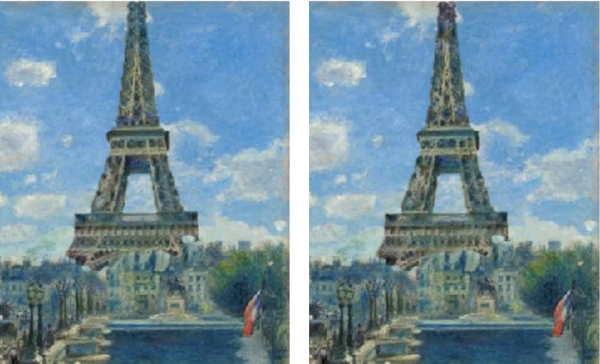
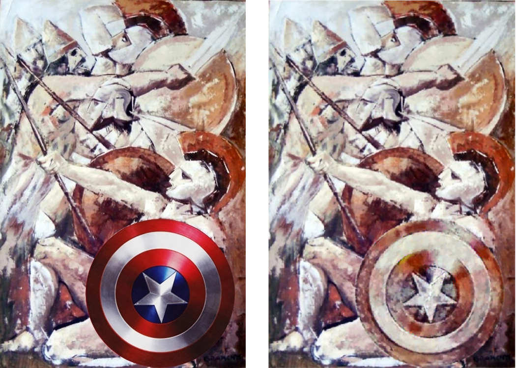
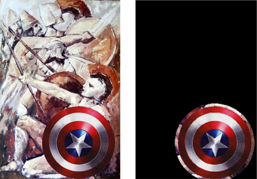
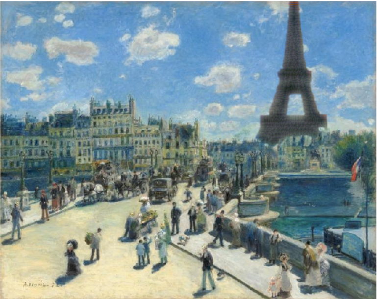
In this article we'll decode this article and get some cool results integrating random objects in paintings while preserving their style like this

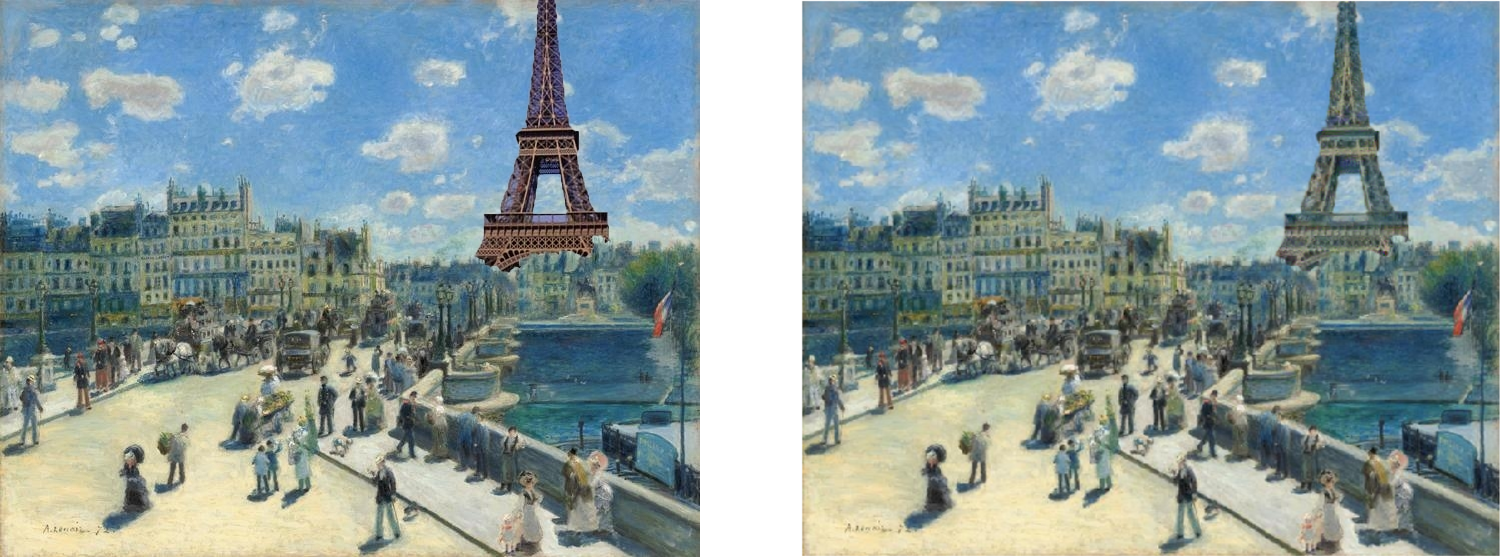
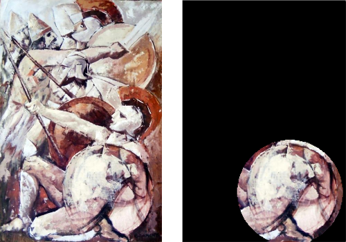
or like this

It goes with this notebook where I have tried to replicate the experiments (all images shown in this post come from applying it).

Style Transfer

To read more about the basics of style transfer, I can only recommend the fast.ai course, or this blog post by an international fellow colleague. Since there's a lot to cover, I will assume you are familiar with this. To make things simple, we will try to match in some way (that is going to be defined later) the features a CNN computes on our input image with the features it computes on our output image.

The model the team who wrote the article chose is VGG19. However, I found similar results with VGG16 which is a bit faster, and lighter in terms of memory, so I used this one. Then we will grab the results of five convolutional layers, the first one and the ones just after the MaxPooling layers (where we half the resolution). The idea is that each will give us some different kind of information. The first convolutional layer is very close to the image, so it will focus more on the details, while the fifth one will be more conceptual and its activation will represent general properties of the picture.

Now to properly integrate the new object in the painting, the authors of the article propose to make two different phases. The first one will focus more on the general style, giving an intermediate result that where the object will still stand out a bit in the picture. The second phase will focus more on the details, and smoothening the edges that could have appeared during the first part. Here is an example of the result of the two stages.

Before going further, a bit of vocabulary. As in the article, we'll call the content picture the painting with our object pasted on it and the style picture the original painting. The input is the content picture for phase 1, the result of this first stage for phase 2. In both cases, we'll compute the results of the convolutional layers for the content picture and the style picture at first, which will serve as our reference features. Then we compute the results of the same convolutional layers for our input, compare them to these references and calculate a loss from that.

At this point, it's all a matter of classic training: we'll compute the gradients of this loss and use them to get a better input, then reiterate the process. As long as our loss properly represents what we want (the object transformed to the style of the painting), we should get some good result. Since the number of parameters is way less than usual (only the pixels of our input compared to all the weights of a model, usually) we can use a variant of SGD that will not only calculate the gradients, but the second derivative as well (the hessian matrix). Without going into the details, this will allow us to make smarter steps each time we update our input, and converge a lot faster. Specifically, we'll use the LBFGS optimizer which is already implemented in pytorch.

This all seems pretty straightforward, but that's because we didn't get to the tough part yet: what are these two magical loss functions (one for stage 1 and one for stage 2) that we will use?

The first pass

The loss function used in this pass is exactly the same as in the original work of Gatys et al. There is a content loss, that measures the difference between our input and the content image, a style loss, that measures the difference between our input and the style image, and we sum them with certain weights to get our final loss.

The main difference is that the article was intended to match a whole picture with a certain style, whereas we only have to worry about part of the picture, the object we add. That means we will mask all the parts of the image that have nothing to do with it when we compute our loss.

In practice, we will use a slightly dilated mask, that encircles a bit more than just the object we're adding (as the authors did in the code they published ). We don't apply that mask before sending the content image, the style image or the output image in the model, which would make us loose information too early, but we resize it to match the dimensions of our different features (the results from the convolutional layers) and apply it to those.

The content loss is then pretty straightforward: it's the mean-squared error between the masked features of our content image and the masked features of our input. The authors chose to use the result of the fourth convolutional layer only for this content loss. Using one of the first convolutional layers would force the final output to match the initial object too closely.

The style loss is a bit trickier. We'll use Gram matrices like we do for regular style transfer, but the problem of the mask is that it might hide some useful information regarding the style. For the content, all the details we needed were inside the mask, because that's where the object we are adding is, but the general style of the painting is more global. That's why before we apply the mask to the style features, we will make some kind of matching to reorganize them.

To be more specific, for each layer of results we have from our model, we'll look at each 3 by 3 (by the number of channels) part of the content features (or patch, as they call it in the article) and find the 3 by 3 patch in the style features that looks the most like it, and match them. To measure how much two patches look alike, we'll use the cosine similarity between them.

Once that mapping is done (note that it is done once and for all between the content and the style), we will transform the style features so that the centers of each 3 by 3 patch in the content features is aligned with its match in the style features. Then we will apply the resized mask on the input features and the style features, compute the Gram matrices of both of them then take the mean-squared error to give us the style loss. The authors chose to use the convolutional layers number 3, 4 and 5 for this style loss, and take the mean of the three of them.

The final loss of this first stage is then:

\begin{equation*} \mathcal{L} = 5 \mathcal{L}_{content} + 100 \mathcal{L}_{loss} \end{equation*}

Once we're done with the construction of our input (they use 1000 iterations in the paper), we make a mean between our output and the style picture to have our final output. We could just use the mask around our object, but that will get an abrupt transition that will stand out, so we use a Gaussian blurring on the sides of the mask (so that we get from the 1s to the 0s a it more smoothly), then compute

\begin{equation*} \hbox{final output} = \hbox{blurred mask} \times \hbox{output} + (1 - \hbox{blurred mask}) \times \hbox{style picture}. \end{equation*}

The second pass

As good as the results of the first pass already are, they usually have two defaults that make the object we added in the painting stand out: first we didn't use any of the features of the first convolutional layers so the fine details, especially those of the painting style, won't be present. Then we didn't do anything to make sure our final picture is smooth.

To remedy to those two things, the authors propose to do a second pass to refine the first result. The first change is in the matching process. This time, the matching between the content and the style is done on a reference layer first, and the results will be transported to the others, but this mapping won't be different for each layer like in the first pass. Then, after doing the first mapping between the content and the style for this reference layer like in the first stage, they refine it by trying to insure that adjacent vectors in the style features remain adjacent through the mapping.

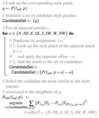
For each pixel p, we consider a certain set of candidates built by going in every direction on p' (in the code they take the full 5 by 5 square centered on p), taking the value given by our first match, and applying to it the inverse of the translation that goes from p to p'. Then we find the candidate that minimizes the L2 loss between its style features and the ones of its neighbors.

Once that matching is done for the reference layer (the authors chose the fourth one), we resize it for the other layers, then proceed like in the first stage to compute the style loss. There is just one difference, they indicate in their article that they suppress the repetitions of the style vectors picked more than once. This is possible because the Gram matrix doesn't care about the exact spacial location of a style feature (since we sum other all locations for each coefficient) but having too many times the same style vectors apparently hurt a bit the performance.

The matching being done, the authors use this time the convolutional layers number 1, 2, 3 and 4 for the style loss (and take the mean of them), and the fourth convolutional layer for the content loss. To add more details to the final output, they also consider two more losses. The first one, the Total Variation loss, just sums the difference between adjacent pixel values, which will insure the result is smoother:

\begin{equation*} \mathcal{L}_{tv} = \sum_{x,y} ((O_{x,y} - O_{x-1,y})^{2} + (O_{x,y} - O_{x,y-1})^{2}) \end{equation*}

where O designs our output. The last one is the histogram loss introduced in this other article .

The histogram loss

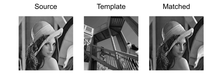
Histogram matching is a technique that is often used to modify a certain photograph with the luminosity or shadows of another. The technique in itself is explained on wikipedia and here is a concrete example of application.

In their paper, Pierre Wilmot et al. found that applying the same technique to define another loss could help preserve the textures of the style picture. They recommended to use it for the features of the first convolutional layer and the fourth one, for both the fine details and the more general aspects of the style.

The idea is, for these two layers, to compute the histogram of each channel of the style features as a reference. Then, at each pass of our training, we calculate the remapping of our output features so that their histogram (for each channel) matches the style reference. We then define the histogram loss as being the the mean-squared error between the output features and their remapped version. The challenge here is to compute that remapping.

Let's say we are trying to change x so that it matches an histogram hist. We sort x first, while keeping the permutation we had to do (it will be used at the end to put the new values we interpolate in their right place). Then, when we treat the i-th value, we look at the first index idx such has hist.cumsum(idx) is greater than i (which means the i-th value of the data we are trying to match the histogram is in the bin with index idx). The value attributed to x[i] is basically

\begin{equation*} \hbox{min} + \hbox{idx} \times \frac{\hbox{max} - \hbox{min}}{n_{bins}} \end{equation*}

where \(\hbox{min}\) and \(\hbox{max}\) are the minim and the maximum values of the data. This formula is slightly corrected because if we have several values of x with the same index idx, we want them to be evenly distributed inside the range of the bin. So we compute the ratio

\begin{equation*} \hbox{ratio} = \frac{i - \hbox{hist.cumsum}(\hbox{idx}-1)}{\hbox{hist}[\hbox{idx}]} \end{equation*}

and finally put

\begin{equation*} x[i] = \hbox{min} + (\hbox{idx} + \hbox{ratio} ) \times \frac{\hbox{max} - \hbox{min}}{n_{bins}}. \end{equation*}

Now we just have to do this for all the i possibles and all the channels. Of course, a simple for loop just won't do if we want to use the GPU to handle all the computations quickly (and if we want 1000 iterations we better compute this remapping as quickly as we can). Let's assume we have our input x of size ch (for channels) by a given n (the number of activations we keep) and a variable hist_ref of size ch by n_bins (they picked 256 in the paper). Sorting x for each channel and keeping the corresponding mapping is easy with pytorch:

sorted_x, sort_idx = x.data.sort(1)

Then we have to adapt our histogram a bit because x and our reference may not have the same number of activations (we removed some style features, the one that appeared more than once). So an histogram for x would have a total sum of n, so we just have to compute the sum of each lines in hist_ref.

hist = hist_ref * n/hist_ref.sum(1).unsqueeze(1)#Normalization between the different lengths of masks.
cum_ref = hist.cumsum(1)
cum_prev = torch.cat([torch.zeros(ch,1).cuda(), cum_ref[:,:-1]],1)

The cumsums will be used later, and we will need both the cumulative sums of hist_ref and the one that contain the cumulative sums for the previous index. To replace our for loop we will create a tensor that contains all the values i from 1 to n. To determine the first index idx such that hist.cumsum(idx) is greater than i, I've used this line:

rng = torch.arange(1,n+1).unsqueeze(0).cuda()
idx = (cum_ref.unsqueeze(1) - rng.unsqueeze(2) < 0).sum(2).long()

Since all the lines of cum_ref are sorted by ascending values, by subtracting i, the sum over the booleans corresponding to the test cum_ref - i < 0 will give us the first index where cum_ref is greater than i. Then we use this tensor idx to get all the values in cum_prev and hist that we will need. Since pytorch doesn't like indexing with a multi-dimensional tensor, we have to flatten everything (though that probably won't be needed anymore in pytorch 0.4)

ymin, ymax = x.data.min(1)[0].unsqueeze(1), x.data.max(1)[0].unsqueeze(1)
step = (ymax-ymin)/n_bins
ratio = (rng - cum_prev.view(-1)[idx.view(-1)].view(ch,-1)) / (1e-8 + hist.view(-1)[idx.view(-1)].view(ch,-1))
ratio = ratio.squeeze().clamp(0,1)
new_x = ymin + (ratio + idx.float()) * step

At this stage new_x contains all the values of our remapping, but they are sorted. We have to use the inverse permutation of the one we applied at the beginning to finish the process. To find the inverse permutation I've simply chose to get the arg sort:

_, remap = sort_idx.sort()
new_x = new_x.view(-1)[remap.view(-1)].view(ch,-1)

Normalization

In the end, the biggest challenge I faced while working on the implementation of this article is the imbalance between the style features and the input features: in the second phase, the mask applied to the style features and the one applied to the input features are different, so the gram matrices we compute from them have different ranges of values. I haven't really understood the way the authors of the paper dealt with this in their code so I chose my own approach.

If we apply a mask with \(n_{1}\) elements for the style features and a mask with \(n_{2}\) elements for the input features, I decided to multiply the style features by \(\sqrt{\frac{n_{2}}{n_{1}}}\) to artificially resize them. Why? Well the gram matrix is computed by doing a sum, which will either have \(n_{1}\) or \(n_{2}\) elements, of products of two elements of our features. So inside that sum, when we compute the gram matrix of the style features, the square root will disappear and we will multiply the result by \(\frac{n_{2}}{n_{1}}\), which is a way to resize this sum of \(n_{1}\) elements to a sum of \(n_{2}\) elements.

Without this little trick, trainings usually gave me this:

For the histograms, we also have a resize to do, which is just done by multiplying the histogram of the style features by this ratio \(\frac{n_{2}}{n_{1}}\). Then in the article they used the minimum and maximum values of the style features to reconstruct the remapped output features, which didn't make any sense to me, since the histogram loss then compares those remapped features to the output features, so I used the minimums and maximums of the output features.

At the end, those four losses are summed with some weights to give the final loss of the second stage:

\begin{equation*} \mathcal{L} = \mathcal{L}_{c} + w_{s} \mathcal{L}_{s} + w_{h} \mathcal{L}_{hist} + w_{tv} \mathcal{L}_{tv} \end{equation*}

where they determine a parameter \(\tau\) by training a neural net they call a painting estimator then use

\begin{equation*} \left \{ \begin{array}{l} w_{s} = \tau \\ w_{tv} = \frac{10 \tau}{(1 + \exp(10^{4} \hbox{mtv} -25))} \\ w_{h} = (10 - w_{tv}) * \tau \end{array} \right . \end{equation*}

I've taken the formulas used in their code, which are different from the ones they put in their article. The quantity mtv is the median of all the variational looses (the things we sum to compute TV loss) on the style picture. Of course, the values of tau that worked for them aren't necessarily the best ones since I've used different scaling for the losses. There are probably some better values that could be used. I didn't get the histogram loss to show any real contribution to the picture, for instance.

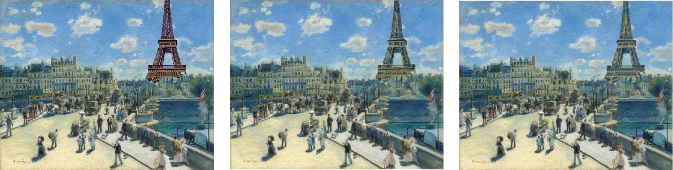
Lastly, for the last stage, we use the result from the first stage to compute the remapping but it's slightly better to use the initial input image for the reconstruction (which the authors do in their code). See the top of the Eiffel tower here, on the left by reconstructing from the input picture and on the right from the stage one.